Introduction
to Microsoft Excel
|
M
|
icrosoft Excel is a powerful spreadsheet
software program that allows making quick & accurate numerical
calculations. Entering data into a spreadsheet is quick & easy. Once you
have entered the data into the worksheet, Excel can instantly perform any type
of calculations on it. The advantage of spreadsheet is that one number is changed;
every number that depends on it is recalculated automatically & changes as
well. Excel can make your information sharp & professional. The uses for
Excel are limitless; business use Excel for creating financial reports,
scientists use Excel for statistical analysis, families may use Excel to help
manage their investment portfolios. . It is an area
with large number of rows (1048576) & column (16384)
How to
start Ms Excel
1st Methord
1. Click on the Start button
2. Highlight Programs
3. Highlight Microsoft Office
4.
Click on Microsoft Excel 2010
2nd Methord
Double click on the desktop Ms Excel
shot cut Icon
3rd Methord.
1.Start
2.Run
3.Type
Excel
How to Exit Excel
1st Methord
1. Click the file tab
2. Click Exit Excel
2nd Methord
Click the close button on the title
bar
3rd Methord
Press Alt key + F4 key
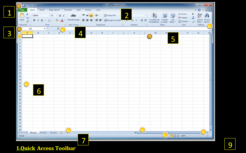
To know the excel 2010 screen elements
|
|
|
|
|
1
|
|
|
|
|
|
3
|
1.Quick Access Toolbar
A Small Toolbar up to the Ribbon
contains short cuts for some of the most common commands such as save, undo,
and redo buttons. You also can customize quick Access toolbar.
2.Ribbon
A Combination of old versions
menu Bar and toolbar, arranged in to series of tabs ranging from home through
view. Each tab contains buttons, lists and commands.
3.Name Box
Displays the
address of the current active cell where you work in the work sheet.
4.Formula bar
Displays the
address of the active cell on the left edge, and it also shows you the current
cell’s contains.
5.column
headings
This area contains
all the cells of the current work sheet identified by column headings, using
letters along the top,
6.row headings
row heading, using
numbers along the left edge with tabs for selecting new work sheets.
7.Sheet tabs
Excel 2010
contains three blank work sheets tabs by default. Click on the intended tab
will go to the particular worksheet.
8.Status bar
Reports information
about the worksheet and provides shortcuts for changing the view and the zoom.
9.Zoom control
Use to zoom the
excel screen in or out by dragging the slider.
To understand tabs
on the excel 2010 Ribbon
File Tab
Open the backstage view of your work
book, where you can open and save files, Get information about the current
workbook, and perform other tasks that do not have to o with the content of the
work book such as printing it or sending a copy of it in e-mail.
Home Tab
This is the most
used tab; it incorporates all text and cell formatting features such as font
and paragraph changes. The Home Tab also includes basic spreadsheet formatting
elements such as text wrap, merging cells and cell style.
Insert Tab
This tab allows
you to insert a variety of items into a document from pictures, clip art, and
headers and footers.
Page Layout Tab
This tab has commands to adjust
page such as margins, orientation and themes.
Formulas Tab
This tab has
commands to use when creating Formulas. This tab holds an immense function
library which can assist when creating any formula or function in your
spreadsheet.
Data Tab
This tab allows
you to modifying worksheets with large amounts of data by sorting and filtering
as well as analyzing and grouping data.
Review Tab
This tab allows
you to correct spelling and grammar issues as well as set up security
protections. It also provides the track changes and notes feature providing the
ability to make notes and changes someone’s document.
View Tab
This tab allows you to change the
view of your document including freezing or splitting panes, viewing gridlines
and hide cells.
Microsoft excel 2010 Workbook and worksheet
A worksheet is the grid of cells where you can type the
data. The grid divides your worksheet in to rows and columns. columns are
identified with letters ( A,B,C…..) ,while rows are identified with numbers
(1,2,3,……). A cell is identified by column and row. For example, B8 is the
address of a cell in column B (the second column), and row 8 (the eighth row).
A work sheet in excel 2010 consists
of columns and over 1 million rows. The worksheets in turn
are grouped together into a workbook. By default each workbook in Excel 2010
contains 3 blank worksheets, which are identified by tabs displaying along the
bottom of your sceen. By
Create a New Workbook
1. Click the File tab
2. click New.
3. Under Available Templates,
double click Blank Workbook or
4. Click Create.
Create a workbook Template
Excel 2010 allows
you to apply built-in templates and to search from a variety of templates on
Office.com. To find a template in Excel 2010, do the following:
1. On
the File tab, click New.
2. Under Available
Templates, do one of the following:
a. To reuse a template that you’ve recently
used, click Recent Templates, click the template that you want, and then
click Create.
b. To
use your own template that you already have installed, click My Templates,
select the template that you want, and then click OK.
c. To find a template on Office.com,
under Office.com Templates, click a template category, select the
template that you want, and then click Download to download the template
from Office.com to your computer.
3. Once you click
on the template you like it will open on your screen as a new document.
Enter Data in a Worksheet
1. Click the cell
where you want to enter data.
2.
Type the data in the cell.
3. Press enter or
tab to move to the next cell.
Select Cells or Ranges
In order to
complete more advanced processes in Excel you need to be able to highlight or
select cells, rows and columns. There are a variety of way to do this, see the
table below to understand the options.
|
To select
|
Do this
|
|
A single cell
|
Click the cell, or press the arrow keys to move to the
cell.
|
|
A range of cells
|
Click the first cell in the range, and then drag to the
last cell, or hold down SHIFT while you press the arrow keys to extend the
selection.
|
|
A large range of cells
|
Click the first cell in the range, and then hold down SHIFT
while you click the last cell in the range. You can scroll to make the last
cell visible.
|
|
All cells on a worksheet
|
Click the Select All button or press CTRL+A.
|
|
Nonadjacent cells or cell ranges
|
Select the first cell or range of cells, and then hold down
CTRL while you select the other cells or ranges.
You cannot cancel the selection of a cell or range of cells
in a nonadjacent selection without canceling the entire selection.
|
|
An entire row or column
|
Click the row or column heading.
Row heading
Column heading
|
|
Adjacent rows or columns
|
Drag across the row or column headings. Or select the first
row or column; then hold down SHIFT while you select the last row or column.
|
|
Nonadjacent rows or columns
|
Click the column or row heading of the first row or column
in your selection; then hold down CTRL while you click the column or row
headings of other rows or columns that you want to add to the selection.
|
|
Cells to the last used cell on the
worksheet (lower-right corner)
|
Select the first cell, and then press CTRL+SHIFT+END to
extend the selection of cells to the last used cell on the worksheet
(lower-right corner).
|
|
Cells to the beginning of the worksheet
|
Select the first cell, and then press CTRL+SHIFT+HOME to
extend the selection of cells to the beginning of the worksheet.
|
Modifying
Spreadsheets
In order to create
an understandable and professional document you will need to make adjustments
to the cells, rows, columns and text. Use the following processes to assist
when creating a spreadsheet.
Cut,
Copy, and Paste Data
You can use the
Cut, Copy, and Paste commands in Microsoft Office Excel to move or copy entire
cells or their contents. Excel displays an animated moving border around cells
that have been cut or copied. To cancel a moving border, press ESC.
Move/Copy Cells
1.
Select the cells that you want to move or copy.
a. To move cells,
click Cut .
b. To copy cells,
click Copy .
3. Click in the
center of the cell you would like to Paste the information too.
4. On the Home
tab, in the Clipboard group, click Paste .
Excel replaces
existing data in the paste area when you cut and paste cells to move them.
Move/Copy Cells with Mouse
1.
Select the cells or a range of cells that you want to move or copy.
2. To move a cell or range of cells, point to the border of
the selection. When the pointer becomes a move pointer
, drag the cell or
range of cells to another location.
Column Width and Row Height
On a worksheet,
you can specify a column width of 0 to 255 and a row height of 0 to 409. This
value represents the number of characters that can be displayed in a cell that
is formatted with the standard font. The default column width is 8.43
characters and the default row height is 12.75 points. If a column/row has a
width of 0, it is hidden.
Save a Spreadsheet
To save a document
in the format used by Excel 2010 and Excel 2007, do the following:
1. Click the File tab.
2. Click Save As.
3. In the File name box, enter a
name for your document.
4. Click Save.
To save a document so that it is
compatible with Excel 2003 or earlier, do the following:
1. Click the File tab.
2. Click Save As.
3. In the Save as type list, click Excel
97-2003 Document. This changes the file format to .xls.
4. In the File name box, type a
name for the document.
5. Click Save.
How to Create Loan/Billing /Time line ….
Templates
1. Click Office
Button / File menu
2. Select New
3. Click Sample
Templates(2010)/Install Templates (2007)
4. Select your
want Templates
5. Click Create
Button
How to check Spelling / Grammar Errors
1. Click Review
tab
2. Select
Proofing Group
3. Click
Spelling And Grammar
4. Select
Suggestions Word
5. Change
Button or Ignore
Insert
worksheet
1. click Home tab,
2.
select
in the Cells group,
3.
click Insert button
4. click Insert Sheet.
Or
1.
Mouse right-click the tab of an
existing worksheet,
2.
click Insert.
3.
Click
General tab
4.
Select Worksheet
5.
Click OK.
Insert Multiple
Worksheets At Once
1.
Hold down SHIFT, and then select the same number of existing sheet tabs
of the worksheets that you want to insert in the open workbook.
2. click On the Home tab,
3. select in the Cells group,
4. click Insert,
5.
Click Insert Sheet.
Or
1.
Mouse
right-click the selected sheet tabs
2.
Click Insert.
3.
Click On the General tab
4.
Click Worksheet
5.
Click OK.
1. click On the Sheet tab bar,
2.
mouse right-click the sheet tab that
you want to rename
3.
click Rename.
4.
Select the current name, and then type
the new name.
or
1.
click On the Home tab,
2.
select
the Cells group,
3.
click the format,
4.
Select rename sheet.
5.
Select the current name, and then type
the new name.
Delete A Worksheet
1.
Click On the Home tab,
2.
Select
the Cells group,
3.
Click the arrow next to Delete, and
then click Delete Sheet.
Or
1.
Mouse right click the sheet tab of the worksheet that you want
to delete,
2.
Click Delete.
Set A Column To A
Specific Width
1.
Select the column or columns that you want to change.
2. click On the Home tab,
3. select in the Cells group,
4.
Click Format.
5.
Under Cell Size, click Column Width.
6.
In the Column width box, type the value
that you want.
To change the width of one column/row
1. Place you cursor on the line between
two rows or columns.
2. . A symbol that looks like a lower case
t with arrows on the horizontal
line will appear
3. Drag the boundary on the right side of
the column/row heading until the
column/row
is the width that you want
1.
Select the column or columns that you want to change.
2.
click On the Home tab,
3.
Click Cells group,
4.
Click Format.
5.
Under Cell Size,
6. click AutoFit Column Width.
Or
1.
To quickly autofit all columns on the
worksheet,
2.
click the Select All button and then
double-click any boundary between two column headings.
Match The Column
Width To Another Column
1. Select a cell in the column.
2.
On the Home tab, in the Clipboard
group, click Copy, and then select the target column.
3.
On the Home tab, in the Clipboard
group, click the arrow below Paste, and then click Paste Special.
4.
Under Paste, select Column widths.
Change The Default
Width For All Columns On A Worksheet Or Workbook
Do one of the following:
1.
To change the default column width for
a worksheet, click its sheet tab.
2.
To change the default column width for the entire workbook, right-click
a sheet tab, and then click Select All Sheets on the shortcut menu.
3.
On the Home tab, in the Cells group, click Format.
4.
Under Cell Size, click Default Width.
5.
In the Default column width box, type a
new measurement.
1. Select the row or rows that you want to change.
2. On the Home tab, in the Cells group, click Format.
3.
Under Cell Size, click Row Height.
4.
In the Row height box, type the value
that you want.
Change The Row Height To Fit The Contents
1.
Select the row or rows that you want to change.
2.
On the Home tab, in the Cells group,
click Format.
3.
Under Cell Size, click AutoFit Row
Height.
To ENTER TEXT INTO
A WORKSHEET
- Select the cell in which you want
to enter the text.
- Type in the text/data into the cell.
- Press the Enter key. Text entries are left
aligned by default.
To edit the worksheet cells
- Select the cell
- press F2 key and start modifying
OR simply double-click on a cell that you wish to modify.
- When finish,
- press Enter.
To change the
Excel cell color background
- Highlight the cells that you want
to alter.
- Click Home tab,
- select Font group,
- point Fill Color button.
- Click the arrow just to the right
of the Fill Color button
- Select you want to colors
To change the text color
- Highlight the text that you want
to change color.
- Click Home tab,
- select Font group,
- point font Color button.
- Click the arrow just to the right
of the font Color button
- Select you want to colors
Merge or Split Cells
Merge and Center Cells
1. Select two or more adjacent cells that you want to merge.
2. On the Home tab, in the Alignment group,
click Merge and Center.
3. The cells will be merged in a row or column, and the cell contents
will be centered in the merged cell.
Merge Cells
1.
Select
Cell
2.
Click home
tab
3.
Selct alignment group
4.
click Merge
Across or Merge Cells.
Split Cells
1. Select the merged cell you want to
split
2. Click home tab
3. Selct
alignment group
4. To split the merged cell, click Merge
and Center
. The cells will
split and the contents of the merged cell will appear in the upper-left cell of
the range of split cells.
Automatically Fill Data
To quickly fill in
several types of data series, you can select cells and drag the fill handle.
To use the fill handle, you select the cells
that you want to use as a basis for filling additional cells, and then drag the
fill handle across or down the cells that you want to fill.
1. Select the cell
that contains the formula that you want to be brought to other cells.
2.Move your curser
to the small black square in the lower-right corner of a selected cell also known
as the fill handle. Your pointer will change to a small black cross.
3. Click and hold your mouse then drag the fill handle across
the cells, horizontally to the right or vertically down, that you want to fill.
4. The cells you want
filled will have a gray looking border around them. Once you fill all of the
cells let go of your mouse and your cells will be populated.
Formatting
Spreadsheets
To further enhance
your spreadsheet you can format a number of elements such as text, numbers,
coloring, and table styles. Spreadsheets can become professional documents used
for company meetings or can even be published.
Wrap Text
1.
Click the cell in which you want to wrap the text.
2. On
the Home tab, in the Alignment group, click Wrap Text.
3. The text in
your cell will be wrapped.
Format Numbers
In Excel, the format of a cell is separate
from the data that is stored in the cell. This display difference can have a
significant effect when the data is numeric. For example, numbers in cells will
default as rounded numbers, date and time may not appear as anticipated. After
you type numbers in a cell, you can change the format in which they are
displayed to ensure the numbers in your spreadsheet are displayed as you
intended.
1.
Click the cell(s) that contains the numbers that you want to format.
Number
Format box, and then
click the format that you want.
If you are unable
to format numbers in the detail you would like that you can click on the More
Number Formats at the bottom of the Number Format drop down list.
1. In the Category list, click the format that
you want to use,and then adjust settings to the right of the Format Cells
dialog box. For example, if you’re using the Currency format, you can select a
different currency symbol, show more or fewer decimal places, or change the way
negative numbers are displayed.
Cell Borders
By using
predefined border styles, you can quickly add a border around cells or ranges
of cells. If predefined cell borders do not meet your needs, you can create a
custom border.
Apply Cell Borders
1. On
a worksheet, select the cell or range of cells that you want to add a border
to, change the border style on, or remove a border from.
2. Go
to the Home tab, in the Font group
3.
Click the arrow next to Borders
4.
Click on the border style you would like
5. The border will
be applied to the cell or cell range
To apply a custom
border style, click More Borders. In the Format Cells dialog box,
on the Border tab, under Line and Color, click the line
style and color that you want
Remove Cell Borders
1. Go to the Home
tab, in the Font group
2. Click the arrow
next to Borders
3. Click No
Border .
The Borders button
displays the most recently used border style. You can click the Borders button
(not the arrow) to apply that style
.
Cell Styles
You can create a
cell style that includes a custom border, colors and accounting formatting.
1. On
the Home tab, in the Styles group, click Cell Styles.
2.
Select the different cell style option you would like applied to your
spreadsheet.
Cell and Text Coloring
You can also
modify a variety of cell and text colors manually.
Cell Fill
1.
Select the cells that you want to apply or remove a fill color from.
2. Go
to the Home tab, in the Font group and select one of the
following
options:
a. To
fill cells with a solid color, click the arrow next to Fill Color
, and then under Theme
Colors or Standard Colors, click the color that you want.
b. To
fill cells with a custom color, click the arrow next to Fill Color
, click More Colors, and then in the Colors dialog
box select the color that you want.
c. To apply the most recently selected color,
click Fill Color
Microsoft Excel
saves your 10 most recently selected custom colors. To quickly apply one of
these colors, click the arrow next to Fill Color , and then click the
color that you want under Recent Colors.
Remove
Cell Fill
1.
Select the cells that contain a fill color or fill pattern.
2. On
the Home tab, in the Font group, click the arrow next to Fill
Color, and then click No Fill.
Text Color
1.
Select the cell, range of cells, text, or characters that you want to format
with a different text color.
2. On the Home tab,
in the Font group and select one of the following options:
a. To apply the most recently selected
text color, click Font Color.
b. To
change the text color, click the arrow next to Font Color,
and then under Theme Colors or Standard Colors, click
the color that you want to use.
Bold, Underline and Italics Text
1.
Select the cell, range of cells, or text.
2. Go
to the Home tab, in the Font group
4. The selected
command will be applied.
Customize Worksheet Tab
1. On
the Sheet tab bar, right-click the sheet tab that you want to customize
2.
Click Rename to rename the sheet or Tab Color to select a tab
color.
3.
Type in the name or select a color you would like for your spreadsheet.
4. The information will be added to the tab at the bottom of
the spreadsheet.
Formula
Formulas
are equations that perform calculations on values in your worksheet. A formula always
starts with an equal sign (=). An example of a simple is =5+2*3 that
multiplies two numbers and then adds a number to the result. Microsoft Office
Excel follows the standard order of mathematical operations. In the preceding
example, the multiplication operation (2*3) is performed first, and then 5 is
added to its result.
In Ms Excel 2010 operators are
executed in this order.
1. Parenthesis ()
2. Percent %
3.
Exponentiation ^
4. Multiplication *
5. Division /
6. Addition _
7. Subtraction -
8. Equal To =
9. Greater Than >
10.
Less Than <
Formula error massagers.
#### The contents of the cell cannot be displayed
correctly as the cell column is too
narrow.
#
REF! Indicates that a cell references is
invalid.
#NAME?
Excel does not recognize text
contained within a formula.
Excel has over 300 built-in functions
divided into various function categories, including:
1.Logical
2.Text
3.Date& Time
4.Lookup Reverence
5.Math Trigonometry
6.Auto Sum
7.Recently Used
8.More Function-:
Logical Functions
AND Returns TRUE
if all of its arguments are TRUE.
FALSE Returns the logical value FALSE.
IF Specifies a logical test to perform.
NOT Reverse the logic of its argument.
OR Retunes true if any argument is TRUE.
TRUE Returns the logical value TRUE.
Statistical Functions.
AVERAGE Returns
the average of its argument.
AVERAGEA Returns
the average of its argument, including numbers, text, and logical values
COUNT Count
how many values are in the list of arguments.
COUNTA Count
how many values are in the list of argument.
MAX Returns
the maximum value in a list of argument.
MEDIAN Returns the median of the given
numbers.
MIN Returns
the minimum value in a list of argument.
RANK Returns the rank of a number in a list of numbers.
Text Functions.
CONCATENATE Joins several text items into one text item.
EXACT Check to see if two text value
are identical.
LOWER converts text to lowercase.
UPPER converts text to uppercase.
PROPER Capitalizes the first letter in each
word of text.
REPT Repeats text a given number of times.
Math & Trigonometry Functions.
SUM Adds
its arguments.
SUMIF Adds the cells specified by a given
criteria.
EVEN Rounds a number up to the nearest
even integer.
INT Rounds a number down to the
nearest integer.
MOD Returns the remainder from
division.
RAND Returns a random number between 0
and 1.
Date & Time Functions.
DATE Returns the serial number of a particular date.
YEAR converts a
serial number to a year.
MONTH
converts a serial number to a month.
WEEKDAY converts
a serial number to a day of the week.
TODAY Returns
the serial number of today’s date.
DAY Converts a
serial number to a day of the month.
TIME Returns the
serial number of a particular time.
HOUR converts a serial number to an hour.
MINUTE converts a serial number to a
minute.
NOW Returns the serial number of current date &
time.
SECOND Converts
a serial number to a second.
DATEVALUE Converts
a date in form of text to serial number.
Database
Functions.
DEAVERAGE Returns the average of selected database
entries.
DCOUNT Counts the cells that contain
numbers in a database.
DMAX Returns the maximum value
from selected database entries.
DSUM Adds the
number in the field column of records in the database that match the criteria.
1. Functions A function, such as PI() or SUM(),
starts with an equal sign (=).
2. Cell
references You can refer to
data in worksheet cells by including cell references in the formula. For
example, the cell reference A2 returns the value of that cell or uses
that value in the calculation.
3. Constants You can also enter constants, such as
numbers (such as 2) or text values, directly into a formula.
4. Operators Operators are the symbols that are used
to specify the type of calculation that you want the formula to perform.
|
EXAMPLE FORMULA
|
WHAT IT DOES
|
|
=5+2
|
Adds 5 and 2
|
|
=5-2
|
Subtracts 2 from 5
|
|
=5/2
|
Divides 5 by 2
|
|
=5*2
|
Multiplies 5 times 2
|
|
=5^2
|
Raises 5 to the 2nd power
|
Create a Simple Formulas
1. Click the cell in which you want to enter the formula.
2. Type = (equal
sign).
3. Enter the formula by typing the constants and operators
that you want to use in the calculation.
4. Press ENTER.
Create a Formula with Cell References
The
first cell reference is B3, the color is blue, and the cell range has a blue border with square
corners. The second cell reference is C3, the color is green, and the cell
range has a green border with square corners.
To create your formula:
1.
Click the cell in which you want to enter the formula.
2. In the formula bar, at the top of the Excel window
that you use
type = (equal sign).
3.
Click on the 1st cell you want in the formula.
4.
Enter an Operator such as +, or *.
5.
Click on the next cell you want in the formula. Continue steps 3 – 5 until the
formula is complete
6. Hit the ENTER
key on your keyboard.
|
EXAMPLE
FORMULA
|
WHAT
IT DOES
|
|
=A1+A2
|
Adds the values
in cells A1 and A2
|
|
=A1-A2
|
Subtracts the
value in cell A2 from the value in A1
|
|
=A1/A2
|
Divides the
value in cell A1 by the value in A2
|
|
=A1*A2
|
Multiplies the value
in cell A1 times the value in A2
|
|
=A1^A2
|
Raises the value
in cell A1 to the exponential value specified in A2
|
Create a Formula with Function
1. Click the cell
in which you want to enter the
2. Click Insert Function
on the formula bar
Excel inserts the equal sign (=) for you.
3. Select the
function that you want to use.
4. Enter the
arguments.
5. After you complete the formula, press ENTER.
Use Auto Sum
To summarize
values quickly, you can also use AutoSum.
1. Select the cell where you would like your
formulas solution to appear.
2. Go
to the Home tab, in the Editing group,
3.
Click AutoSum, to sum your numbers or click the arrow next to AutoSum
to select a function that you want
to apply.
Delete a Formula
When you delete a
formula, the resulting values of the formula is also deleted. However, you can
instead remove the formula only and leave the resulting value of the formula
displayed in the cell.
To delete formulas along with their
resulting values, do the following:
1.
Select the cell or range of cells that contains the formula.
2. Press DELETE.
To delete formulas without removing
their resulting values, do the following:
1.
Select the cell or range of cells that contains the formula.
2. On
the Home tab, in the Clipboard group, click Copy
.
3. On the Home tab, in the Clipboard group,
click the arrow below Paste
and then click Paste Values.
Charts
in Excel
To create a chart
in Excel, you start by entering the numeric data for the chart on a worksheet.
Then you can plot that data into a chart by selecting the chart type that you
want to use on the Insert tab, in the Charts group.
Getting to know the elements of a chart
1 The chart area is the entire chart and all its
elements
2 The plot area is the area of the chart bounded by the
axes.
3
The data points
are individual values plotted in a chart represented by bars, columns, lines, or pies.
4 The horizontal (category) and vertical (value) axis
along which the data is plotted in the chart.
5 The legend identifies the patterns or colors that are
assigned to the data series or categories in the chart.
6 A chart and axis title are descriptive text that for
the axis or chart.
7 A data label provides additional
information about a data marker that you can use to identify the details of a
data point in a data series.
Create a Chart
2. Select the
cells that contain the data that you want to use for the chart.
If the
cells that you want to plot in a chart are not in a continuous range, you can select
nonadjacent cells or ranges as long as the selection forms a rectangle. You can
also hide the rows or columns that you do not want to plot in the chart.
3. Go
to the Insert tab, in the Charts
4.
Click the chart type, and then click a chart subtype from the drop menu that
will appear.
5.
Click anywhere in the embedded chart to activate it. When you click on the
chart, Chart Tools will be displayed which includes the Design,
Layout, and Format tabs.
Move Chart to New Sheet
1. On the Design tab, in the Location
group, click Move Chart.
2. Under Choose where you want the
chart to be placed,
3. click on the New sheet bubble
4. Type a chart name in the New sheet box.
Change Chart Name
1.
Click the chart.
2. On the Layout tab, in the Properties
group, click the Chart Name text box.
3. Type a new chart name.
4. Press ENTER.
1.
Click anywhere in the chart.
2. Go
to the Chart Tools, the Design group
3. In the Chart
Layouts, click the chart layout that you want to use. To see all available
layouts, click
Change Chart Style
1.
Click anywhere in the chart.
2. On the Design tab, in the Chart Styles group,
click the chart style that you want to use. To see all predefined chart styles,
click More
Chart or Axis Titles
To make a chart
easier to understand, you can add titles, such as chart and axis titles.
To add a chart title:
1. Click anywhere
in the chart.
2. On the Layout tab, in the Labels
group, click Chart Title.
3. Click Centered Overlay Title or
Above Chart.
4. In the Chart Title text box
that appears in the chart, type the text that you want.
5. To remove a chart
title, click Chart Title, and then click None.
To add axis titles:
1.
Click anywhere in the chart.
2. On
the Layout tab, in the Labels group, click Axis Titles.
3. Do one or more
of the following:
a. To
add a title to a primary horizontal (category) axis, click Primary Horizontal Axis Title, and then click
the option that you want.
b. To add a title to primary vertical (value) axis, click Primary
Vertical Axis Title, and then click the option that you want.
4. In
the Axis Title text box that appears in the chart, type the text that you want.
Data Labels
1. On a chart, do
one of the following:
a.
Click on the chart area to add a data label to all data points of all
data series
b.
Click in the data series to add a data label to all data points of a
data series
c.
Click on a specific data point to add a data label to a single data
point in a data series
2. On
the Layout tab, in the Labels group, click Data Labels,
and then click the display option that you want.
3.
Text boxes will appear in the area of your chart based on your selection.
4.
Click on the text box to modify the text.
Legend
When you create a
chart, the legend appears, but you can hide the legend or change its location
after you create the chart.
1. Click the chart
in which you want to show or hide a legend.
2. On the Layout
tab, in the Labels group, click Legend.
3. Do one of the
following:
a. To hide the
legend, click None.
b. To display a
legend, click the display option that you want.
c. For additional options, click More
Legend Options, and then select the display option that you want.
Move or Resize
Chart
You can move a chart to any location on a worksheet or to a
new or existing worksheet. You can also change the size of the chart for a
better fit. To move a chart, drag it to the location that you want. To resize a
chart, click on one of the edges and drag towards the center.
Advanced Spreadsheet Modification
Once you have
created a basic spreadsheet there are numerous things you can do to make
working with you data easier. Some of these elements are hiding, freezing and
splitting rows. You can also sort and filter data, these features are quite
helpful when working with a large amount of data.
Hide or Display
Rows and Columns
You can hide a row or column by using the Hide
command or when you change its row height or column width to 0 (zero). You
can display either again by using the Unhide command. You can either
unhide specific rows and columns, or you can unhide all hidden rows and columns
at the same time. The first row or column of the worksheet is tricky to unhide,
but it can be done.
Hide Rows or Columns
1. Select the rows or columns that you want to hide.
2. On
the Home tab, in the Cells group, click Format.
3.
Under Visibility, point to Hide & Unhide, and then click Hide
Rows or Hide Columns.
You can also right-click a row or
column (or a selection of multiple rows or columns), and then click Hide.
Unhide Rows or Columns
1.
Select the rows, columns or entire sheet to unhide.
2. On
the Home tab, in the Cells group, click Format.
3.
Under Visibility, point to Hide & Unhide, and then click Unhide
Rows or Unhide Columns.
Freezing/Splitting Rows and Columns
Freezing vs. splitting
When you split panes,
Excel creates either two or four separate worksheet areas that you can scroll
within, while rows or columns in the non-scrolled area remain visible. This
worksheet has been split into four areas. Notice that each area contains a
separate view of the same data. Splitting panes is useful when you want to see
different parts of a large spreadsheet at the same time. You cannot split panes
and fre eze panes at the same
Freeze Panes
1. On the
worksheet, select the row or column that you want to keep visible when you
scroll.
2. On the View tab,
in the Window group, click the arrow below Freeze Panes.
¨
To
lock one row only, click Freeze Top Row.
¨
To
lock one column only, click Freeze First Column.
¨
To
lock more than one row or column, or to lock both rows and columns at the same
time, click Freeze Panes.
You can freeze
rows at the top and columns on the left side of the worksheet only. You cannot
freeze rows and columns in the middle of the worksheet.
Unfreeze panes
1.
On the
View tab, in the Window group, click the arrow below Freeze
Panes.
2.
Click Unfreeze
Panes.
Split Panes
1. To split panes, point to the split
box at the top of the vertical scroll bar or at the right end of the horizontal
scroll bar.
2. When the pointer changes to a split
pointer or drag the split box down or to the left to the
position that you want.
3. To remove the
split, double-click any part of the split bar that divides the panes.
Moving or Copying Worksheets
Sometimes you may
need to copy an entire worksheet instead of copying and pasting the data which
may or may not paste properly, you can use the steps below to achieve a must
better result.
Move or Copy
Worksheets
1. Select the worksheets that you want to move or
copy.
3. A Move
or Copy dialog box will appear
4. To move a
sheet, in the Before sheet list:
5. To copy the
sheets, in the Move or Copy dialog box, select the Create a copy check box.
Move or Copy to a
Different Workbook
1. In
the workbook that contains the sheets that you want to move or
copy, select the sheets.
2. On
the Home tab, in the Cells group, click Format, and then
under
Organize Sheets, click Move or Copy Sheet.
3. In
the Move or Copy dialog box, click the drop down list in the To
book box, then:
selected sheets.
workbook.
6. To move a
sheet, in the Before sheet list:
7. To copy the sheets, in the Move or Copy dialog box,
select the Create a copy check box.
Create a PivotTable
from worksheet data
When you create a
PivotTable report from worksheet data, that data becomes the source data for
the PivotTable report.
1.
Do
one of the following:
§ To
use worksheet data as the data source, click a cell in the range of cells that
contains the data.
§ To
use data in an Excel table as the data source, click a cell inside the Excel
table.
2.
Click
On the Insert tab,
3.
Select
in the Tables group,
4.
Click PivotTable, or click the arrow
below PivotTable, and then click PivotTable. Excel displays the Create
PivotTable dialog box.
5.
Under
Choose the data that you want to analyze, make sure that Select a
table or range is selected, and then in the Table/Range box, verify
the range of cells that you want to use as the underlying data.
.
6.
Under
Choose where you want the PivotTable report to be placed, specify a
location by doing one of the following:
§ To
place the PivotTable report in a new worksheet starting at cell A1, click New
Worksheet.
§ To
place the PivotTable report in an existing worksheet, select Existing
Worksheet, and then in the Location box, specify the first cell in
the range of cells where you want to position the PivotTable report.
7.
Click
OK.
8.
To
add fields to the report, do one or more of the following:
§ To
place a field in the default area of the layout section, select the check box
next to the field name in the field section.
§ To
place a field in a specific area of the layout section, right-click the field
name in the field section, and then select Add to Report Filter, Add
to Column Label, Add to Row Label, or Add to Values.
§ To
drag a field to the area that you want, click and hold the field name in the
field section, and then drag it to an area in the layout section.
1. Click
the PivotTable report.
This
displays the PivotTable Tools, adding the Options and Design
tab.
2. On
the Options tab, in the Tools group, click PivotChart.
3.
In
the Insert Chart dialog box, click the chart type and chart subtype that
you want. You can use any chart type except an xy (scatter), bubble, or stock
chart.
4.
Click
OK.
Delete a
PivotTable report
1.
Click
anywhere in the PivotTable report that you want to delete.
2.
On
the Options tab, in the Actions group, click the arrow below Select,
and then click Entire PivotTable.
3.
Press
DELETE.
Deleting a PivotTable
report that is associated with a PivotChart report turns that PivotChart report
into a standard chart that you can no longer pivot or update.
Delete a
PivotChart report
1.
Click
anywhere in the PivotChart that you want to delete.
2.
Press
DELETE.
Deleting a PivotChart
report does not delete the associated PivotTable report.
Sorting Data
Sorting data is an
integral part of data analysis. You might want to arrange a list of names in
alphabetical order, compile a list of product inventory levels from highest to
lowest, or order rows by colors or icons. Sorting data helps you quickly
visualize and understand your data better, organize and find the data that you
want, and ultimately make more effective decisions.
Sort Data in
Single Column
1.
Select a column of data in a range of cells
2. On
the Data tab, in the Sort & Filter group, do one of the
following:
3. To
reapply a sort after you change the data, click a cell in the range or
table
and then, on the Data tab, in the Sort & Filter group, click Reapply.
Sort Data in
Multiple Columns or Rows
You may want to
sort by more than one column or row when you have data that you want to group
by the same value in one column or row, and then sort another column or row
within that group of equal values.
1.
Select a range of cells with two or more columns of data.
2. On
the Data tab, in the Sort & Filter group, click Sort.
3. The
Sort dialog box will appear.
4.
Under Column, in the Sort by box, select the first column that
you want to sort.
6. Under Order,
select how you want to sort.
7. To
add another column to sort by, click Add Level, and then repeat steps
four through six.
8. To
copy a column to sort by, select the entry and then click Copy Level.
9. To
delete a column to sort by, select the entry and then click Delete Level.
10 To
change the order in which the columns are sorted, select an entry and then
click the Up or Down arrow to change the order.
11. To reapply a sort after you change the
data, click a cell in the range or table and then, on the Data tab, in
the Sort & Filter group, click Reapply.
- Right-click the
chart legend and choose Font.
- From the Font dialog
box displayed, select the required formatting options.
- Click the OK button.
Advance
Filter
1.
Select data range
2.
Click data tab
3.
In sort & filter group Click
advance filter
4.
Select data rang
5.
Select criteria range
6.
Select copy to
7.
Select action –copy to another
location
8.
Select unique records only
Auto Filter
1.
Select data
range
2.
Click data tab
3.
In sort & filter group click
auto filter
4.
Select criteria
Remove auto filter
1.
Select data range
2.
Click data tab
3.
In sort & filter group click
auto filter
Finalizing
a Spreadsheet
To complete your
spreadsheet there are a few steps to take to ensure your document is finalized.
Excel
does not have the same spell check feature as Word and PowerPoint. To complete
a Spelling and Grammar check, you need to use the Spelling and Grammar feature.
1. Click on the Review tab
2. Click on the Spelling & Grammar command
(a blue check mark with ABC above it).
3. A Spelling and Grammar box will
appear, correct any Spelling or Grammar issue with the help of the box
Print Preview
Print Preview
automatically displays when you click on the Print tab. Whenever you make
a change to a print-related setting, the preview is automatically updated.
1.
Click the File tab, and then click Print. To go back to your
document, click the File tab.
2. A preview of your document automatically appears. To view
each page, click the arrows below the preview.
Print a Worksheet
1. Click the
worksheet or select the worksheets that you want to print.
2. Click File
3.
Click Print.
4. Once you are on the Print screen you can
select printing options:
and select the
printer that you want.
orientation, paper
size, and page margins, select the options
that you want
under Settings.
under Settings,
click the option that you want in the scale
options drop-down
box.
Print Entire
Workbook
5. Click Print.
How
to apply header
1. Click insert tab
2. Select text group
3. Click header & footer button
4. Click header & footer tools
5. Select header & footer elements group
6. Select t you want to element or type
How To Change Worksheet Margins,
1. Click Page Layout tab
2. Select Page Set up Group
3. Click Margins Button
4. Select Suitable Margins
How
to Change Orientation
1. Click Page Layout tab
2. Select Page Set up Group
3. Click Orientation
4. Click Orientation Button
5. Select Portrait or Landscape
How
to Change Paper Size
1. Click Page Layout tab
2. Select Page Set up Group
3. Click Page Size button
4. Select Suitable paper Size
How
to Change Print Area
1. Select Print Area
2. Click Page Layout tab
3. Select Page Set up Group
4. Click Print Area button
5. Click set print area
How
to Remove Print Area
1. Select Print Area
2. Click Page Layout tab
3. Select Page Set up Group
4. Click Print Area button
5. Click set print area
How to insert page breaks
1. Click Page Layout tab
2. Select Page Set up Group
3. Click Break
button
4. Click insert page break
How to remove page breaks
1. Click Page Layout tab
2. Select Page Set up Group
3. Click Break
button
4. Click remove page break
How to add print title
1. Click Page Layout tab
2. Select Page Set up Group
3. Click Print title
button
4. Click sheet tab
5. Select print title using rows to repeat at top
6. Click ok button
How
to print grid line
1. Click Page Layout tab
2. Select sheet option
Group
3. Select view & print grid check box
How to scale page
1. Click Page Layout
tab
2. Select Scale to
fit Group
3. Select Scale
Print a Worksheet
1. Click the
worksheet or select the worksheets that you want to print.
2. Click File
3.
Click Print.
4. Once you are on the Print screen you can
select printing options:
5. Click Print.
Spreadsheet / worksheet settings (magnification / Zoom tools,
tool bar display / hide, row /
• Worksheet Preview function
How to apply column freezing
Help
1. Click on the blue circle with the white
question mark command
2. A Help box
will appear.
3. Click in the Search
Help textbox and type what you need help with
4.
Click the magnifying glass next to the text box and the possible solutions will
appear.
For
additional information Microsoft Office has a great online resource that
provides you with step by step instructions in a variety of topics. This link
will bring you directly to the Word 2010 Help and
No comments:
Post a Comment